2222a,皇弟的失宠新娘,最搞笑的笑话大全
一、bn(batch normalization)算法
1. 对数据进行归一化处理的重要性
神经网络学习过程的本质就是学习数据分布,在训练数据与测试数据分布不同情况下,模型的泛化能力就大大降低;另一方面,若训练过程中每批batch的数据分布也各不相同,那么网络每批迭代学习过程也会出现较大波动,使之更难趋于收敛,降低训练收敛速度。对于深层网络,网络前几层的微小变化都会被网络累积放大,则训练数据的分布变化问题会被放大,更加影响训练速度。
2. bn算法的强大之处
1)为了加速梯度下降算法的训练,我们可以采取指数衰减学习率等方法在初期快速学习,后期缓慢进入全局最优区域。使用bn算法后,就可以直接选择比较大的学习率,且设置很大的学习率衰减速度,大大提高训练速度。即使选择了较小的学习率,也会比以前不使用bn情况下的收敛速度快。总结就是bn算法具有快速收敛的特性。
2)bn具有提高网络泛化能力的特性。采用bn算法后,就可以移除针对过拟合问题而设置的dropout和l2正则化项,或者采用更小的l2正则化参数。
3)bn本身是一个归一化网络层,则局部响应归一化层(local response normalization,lrn层)则可不需要了(alexnet网络中使用到)。
3. bn算法概述
bn算法提出了变换重构,引入了可学习参数γ、β,这就是算法的关键之处:

引入这两个参数后,我们的网络便可以学习恢复出原是网络所要学习的特征分布,bn层的钱箱传到过程如下:

其中m为batchsize。batchnormalization中所有的操作都是平滑可导,这使得back propagation可以有效运行并学到相应的参数γ,β。需要注意的一点是batch normalization在training和testing时行为有所差别。training时μβ和σβ由当前batch计算得出;在testing时μβ和σβ应使用training时保存的均值或类似的经过处理的值,而不是由当前batch计算。
二、tensorflow相关函数
1.tf.nn.moments(x, axes, shift=none, name=none, keep_dims=false)
x是输入张量,axes是在哪个维度上求解, 即想要 normalize的维度, [0] 代表 batch 维度,如果是图像数据,可以传入 [0, 1, 2],相当于求[batch, height, width] 的均值/方差,注意不要加入channel 维度。该函数返回两个张量,均值mean和方差variance。
2.tf.identity(input, name=none)
返回与输入张量input形状和内容一致的张量。
3.tf.nn.batch_normalization(x, mean, variance, offset, scale, variance_epsilon,name=none)
计算公式为scale(x - mean)/ variance + offset。
这些参数中,tf.nn.moments可得到均值mean和方差variance,offset和scale是可训练的,offset一般初始化为0,scale初始化为1,offset和scale的shape与mean相同,variance_epsilon参数设为一个很小的值如0.001。
三、tensorflow代码实现
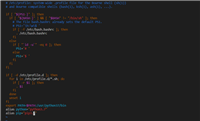
1. 完整代码
import tensorflow as tf
import numpy as np
import matplotlib.pyplot as plt

activition = tf.nn.relu
n_layers = 7 # 总共7层隐藏层
n_hidden_units = 30 # 每层包含30个神经元

def fix_seed(seed=1): # 设置随机数种子
  np.random.seed(seed)
  tf.set_random_seed(seed)

def plot_his(inputs, inputs_norm): # 绘制直方图函数
  for j, all_inputs in enumerate([inputs, inputs_norm]):
    for i, input in enumerate(all_inputs):
      plt.subplot(2, len(all_inputs), j*len(all_inputs)+(i+1))
      plt.cla()
      if i == 0:
        the_range = (-7, 10)
      else:
        the_range = (-1, 1)
      plt.hist(input.ravel(), bins=15, range=the_range, color='#ff5733')
      plt.yticks(())
      if j == 1:
        plt.xticks(the_range)
      else:
        plt.xticks(())
      ax = plt.gca()
      ax.spines['right'].set_color('none')
      ax.spines['top'].set_color('none')
    plt.title("%s normalizing" % ("without" if j == 0 else "with"))
  plt.draw()
  plt.pause(0.01)

def built_net(xs, ys, norm): # 搭建网络函数
  # 添加层
  def add_layer(inputs, in_size, out_size, activation_function=none, norm=false):
    weights = tf.variable(tf.random_normal([in_size, out_size],
                        mean=0.0, stddev=1.0))
    biases = tf.variable(tf.zeros([1, out_size]) + 0.1)
    wx_plus_b = tf.matmul(inputs, weights) + biases

    if norm: # 判断是否是batch normalization层
      # 计算均值和方差,axes参数0表示batch维度
      fc_mean, fc_var = tf.nn.moments(wx_plus_b, axes=[0])
      scale = tf.variable(tf.ones([out_size]))
      shift = tf.variable(tf.zeros([out_size]))
      epsilon = 0.001

      # 定义滑动平均模型对象
      ema = tf.train.exponentialmovingaverage(decay=0.5)

      def mean_var_with_update():
        ema_apply_op = ema.apply([fc_mean, fc_var])
        with tf.control_dependencies([ema_apply_op]):
          return tf.identity(fc_mean), tf.identity(fc_var)

      mean, var = mean_var_with_update()

      wx_plus_b = tf.nn.batch_normalization(wx_plus_b, mean, var,
                         shift, scale, epsilon)

    if activation_function is none:
      outputs = wx_plus_b
    else:
      outputs = activation_function(wx_plus_b)
    return outputs

  fix_seed(1)

  if norm: # 为第一层进行bn
    fc_mean, fc_var = tf.nn.moments(xs, axes=[0])
    scale = tf.variable(tf.ones([1]))
    shift = tf.variable(tf.zeros([1]))
    epsilon = 0.001

    ema = tf.train.exponentialmovingaverage(decay=0.5)

    def mean_var_with_update():
      ema_apply_op = ema.apply([fc_mean, fc_var])
      with tf.control_dependencies([ema_apply_op]):
        return tf.identity(fc_mean), tf.identity(fc_var)

    mean, var = mean_var_with_update()
    xs = tf.nn.batch_normalization(xs, mean, var, shift, scale, epsilon)

  layers_inputs = [xs] # 记录每一层的输入

  for l_n in range(n_layers): # 依次添加7层
    layer_input = layers_inputs[l_n]
    in_size = layers_inputs[l_n].get_shape()[1].value

    output = add_layer(layer_input, in_size, n_hidden_units, activition, norm)
    layers_inputs.append(output)

  prediction = add_layer(layers_inputs[-1], 30, 1, activation_function=none)
  cost = tf.reduce_mean(tf.reduce_sum(tf.square(ys - prediction),
                    reduction_indices=[1]))

  train_op = tf.train.gradientdescentoptimizer(0.001).minimize(cost)
  return [train_op, cost, layers_inputs]

fix_seed(1)
x_data = np.linspace(-7, 10, 2500)[:, np.newaxis]
np.random.shuffle(x_data)
noise =np.random.normal(0, 8, x_data.shape)
y_data = np.square(x_data) - 5 + noise

plt.scatter(x_data, y_data)
plt.show()

xs = tf.placeholder(tf.float32, [none, 1])
ys = tf.placeholder(tf.float32, [none, 1])

train_op, cost, layers_inputs = built_net(xs, ys, norm=false)
train_op_norm, cost_norm, layers_inputs_norm = built_net(xs, ys, norm=true)

with tf.session() as sess:
  sess.run(tf.global_variables_initializer())

  cost_his = []
  cost_his_norm = []
  record_step = 5

  plt.ion()
  plt.figure(figsize=(7, 3))
  for i in range(250):
    if i % 50 == 0:
      all_inputs, all_inputs_norm = sess.run([layers_inputs, layers_inputs_norm],
                          feed_dict={xs: x_data, ys: y_data})
      plot_his(all_inputs, all_inputs_norm)

    sess.run([train_op, train_op_norm],
         feed_dict={xs: x_data[i*10:i*10+10], ys: y_data[i*10:i*10+10]})

    if i % record_step == 0:
      cost_his.append(sess.run(cost, feed_dict={xs: x_data, ys: y_data}))
      cost_his_norm.append(sess.run(cost_norm,
                     feed_dict={xs: x_data, ys: y_data}))

  plt.ioff()
  plt.figure()
  plt.plot(np.arange(len(cost_his))*record_step,
       np.array(cost_his), label='without bn')   # no norm
  plt.plot(np.arange(len(cost_his))*record_step,
       np.array(cost_his_norm), label='with bn')  # norm
  plt.legend()
  plt.show()
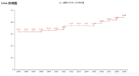
2. 实验结果
输入数据分布:

批标准化bn效果对比:

以上就是本文的全部内容,希望对大家的学习有所帮助,也希望大家多多支持移动技术网。
如对本文有疑问,请在下面进行留言讨论,广大热心网友会与你互动!! 点击进行留言回复

Python 实现将numpy中的nan和inf,nan替换成对应的均值

python爬虫把url链接编码成gbk2312格式过程解析
网友评论