sciket-learn官网链接:https://scikit-learn.org/stable/
sciket-learn官网文档中文版:https://sklearn.apachecn.org/
推荐一本书PRML:PRML为何是机器学习的经典书籍中的经典?- 知乎
scikit-learn,又写作sklearn,是一个开源的基于python语言的机器学习工具包。它通过NumPy, SciPy和Matplotlib等python数值计算的库实现高效的算法应用,并且涵盖了几乎所有主流机器学习算法。
sklearn优点:
常用模块
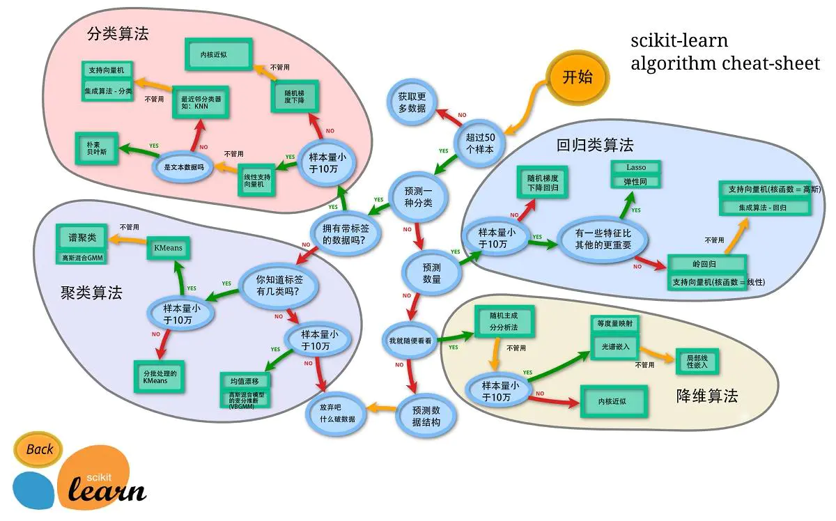
sklearn中常用的模块有分类、回归、聚类、降维、模型选择、预处理。
分类:识别某个对象属于哪个类别,常用的算法有:SVM(支持向量机)、nearest neighbors(最近邻)、random forest(随机森林),常见的应用有:垃圾邮件识别、图像识别。
回归:预测与对象相关联的连续值属性,常见的算法有:SVR(支持向量机)、 ridge regression(岭回归)、Lasso,常见的应用有:药物反应,预测股价。
聚类:将相似对象自动分组,常用的算法有:k-Means、 spectral clustering、mean-shift,常见的应用有:客户细分,分组实验结果。
降维:减少要考虑的随机变量的数量,常见的算法有:PCA(主成分分析)、feature selection(特征选择)、non-negative matrix factorization(非负矩阵分解),常见的应用有:可视化,提高效率。
模型选择:比较,验证,选择参数和模型,常用的模块有:grid search(网格搜索)、cross validation(交叉验证)、 metrics(度量)。它的目标是通过参数调整提高精度。
预处理:特征提取和归一化,常用的模块有:preprocessing,feature extraction,常见的应用有:把输入数据(如文本)转换为机器学习算法可用的数据。
# 基础结构.py
#选模型+调参
import numpy as np
from sklearn import neighbors, datasets, preprocessing# 数据预处理
from sklearn.model_selection import train_test_split# 数据切分
from sklearn.metrics import accuracy_score # 指标评估
from sklearn.model_selection import cross_val_score# 模型选择

np.random.RandomState(0)# # 随机数定下来

# 加载数据
iris = datasets.load_iris()

# 划分训练集与测试集
x, y = iris.data, iris.target
x_train, x_test, y_train, y_test = train_test_split(x, y, test_size=0.3)# 30%做测试集

# 数据预处理
scaler = preprocessing.StandardScaler().fit(x_train)
x_train = scaler.transform(x_train)
x_test = scaler.transform(x_test)

# 创建模型
knn = neighbors.KNeighborsClassifier(n_neighbors=12)

# 模型拟合
knn.fit(x_train, y_train)

# 交叉验证(用在训练的时候)
scores = cross_val_score(knn, x_train, y_train, cv=5, scoring='accuracy')
print(scores)  # 每组的评分结果
print(scores.mean())

# 预测
y_pred = knn.predict(x_test)

# 评估
print(accuracy_score(y_test, y_pred))
from sklearn import datasets
from sklearn.model_selection import train_test_split
from sklearn.neighbors import KNeighborsClassifier
from sklearn.model_selection import cross_val_score#引入交叉验证
import  matplotlib.pyplot as plt
###引入数据###
iris=datasets.load_iris()
X=iris.data
y=iris.target
###设置n_neighbors的值为1到30,通过绘图来看训练分数###
k_range=range(1,31)
k_score=[]
for k in k_range:
    knn=KNeighborsClassifier(n_neighbors=k)
    scores=cross_val_score(knn,X,y,cv=10,scoring='accuracy')#for classfication
    k_score.append(scores.mean())
plt.figure()
plt.plot(k_range,k_score)
plt.xlabel('Value of k for KNN')
plt.ylabel('CrossValidation accuracy')
plt.show()

import numpy as np
import matplotlib.pyplot as plt
from sklearn.model_selection import GridSearchCV
from sklearn.svm import SVR

rng = np.random.RandomState(0)

X = 5 * rng.rand(100, 1)
y = np.sin(X).ravel()

y[::5] += 3 * (0.5 - rng.rand(X.shape[0] // 5))

svr = GridSearchCV(SVR(kernel='rbf'),
                   param_grid={"C": [1e0, 1e1, 1e2, 1e3],
                               "gamma": np.logspace(-2, 2, 5)})
svr.fit(X, y)
print(svr.best_score_, svr.best_params_)

X_plot = np.linspace(0, 5, 100)
y_svr = svr.predict(X_plot[:, None])

plt.scatter(X, y)
plt.plot(X_plot, y_svr, color="red")
plt.show()


构造回归数据集:
import matplotlib.pyplot as plt

from sklearn.datasets.samples_generator import make_regression

# X为样本特征,y为样本输出, coef为回归系数,共1000个样本,每个样本1个特征
x, y, coef = make_regression(n_samples=100, n_features=1, noise=10, coef=True)
print(coef)

# 画图
plt.scatter(x, y)
plt.plot(x, x * coef, color='blue', linewidth=3)

plt.show()

然而,对于普通最小二乘问题,其系数估计依赖模型各项相互独立。当各项是相关的,设计矩阵(Design Matrix) x 的各列近似线性相关, 那么,设计矩阵会趋向于奇异矩阵,这会导致最小二乘估计对于随机误差非常敏感,会产生很大的方差。

MAE反映预测值误差的实际情况。

MSE衡量的是样本整体与模型预测值偏离程度。

可解释方差指标衡量的是所有预测值和样本之间的差的分散程度与样本本身的分散程度的相近程度。本身是分散程度的对比。最后用1-这个值,最终值越大表示预测和样本值的分散分布程度越相近。

R²分数:
指标解读:因变量的方差能被自变量解释的程度
指标越接近1,则代表自变量对于因变量的解释度越高
w过大,模型不稳定
加了一个正则项,对w进行惩罚,α是超参数表示对w惩罚的力度。当w太小,有可能会使损失无法下降


import numpy as np
import matplotlib.pyplot as plt
from sklearn import linear_model

# X 是10x10的希尔伯特矩阵
X = 1. / (np.arange(1, 11) + np.arange(0, 10)[:, np.newaxis])
y = np.ones(10)
print(X)
# 计算不同岭系数时的回归系数
n_alphas = 200
alphas = np.logspace(-10, -2, n_alphas)

coefs = []
for a in alphas:
    ridge = linear_model.Ridge(alpha=a, fit_intercept=False)
    ridge.fit(X, y)
    coefs.append(ridge.coef_)

#绘图
ax = plt.gca()
plt.rcParams['font.sans-serif']=['SimHei']
plt.rcParams['axes.unicode_minus'] = False
ax.plot(alphas, coefs)
ax.set_xscale('log')
ax.set_xlim(ax.get_xlim()[::-1])
plt.xlabel('岭系数alpha')
plt.ylabel('回归系数coef_')
plt.title('岭系数对回归系数的影响',)
plt.axis('tight')
plt.show()


L1、L2正则化混用

输入数据压缩+L1、L2正则化
本质:加了非线性函数(激活函数)


从贝叶斯的角度看:P(W|x,y)=P(Y|x,w)*P(w)/P(x|y,w)

(1)对参数引入 拉普拉斯先验 等价于 L1正则化。
(2)对参数引入 高斯先验 等价于 L2正则化。
(3)正则化参数等价于对参数引入先验分布,使得模型复杂度变小(缩小解空间),对于噪声以及 outliers 的鲁棒性增强(泛化能力)。整个最优化问题从贝叶斯观点来看是一种贝叶斯最大后验估计,其中正则化项对应后验估计中的先验信息,损失函数对应后验估计中的似然函数,两者的乘积即对应贝叶斯最大后验估计的形式。
# LinearRegression.py
# 普通线性回归
from sklearn import linear_model
import matplotlib.pyplot as plt
import numpy as np
from sklearn import datasets
from sklearn.model_selection import train_test_split
from sklearn.metrics import mean_absolute_error, mean_squared_error, r2_score, explained_variance_score

np.random.RandomState(0)

x, y = datasets.make_regression(n_samples=100, n_features=1, n_targets=1, noise=10)
x_train, x_test, y_train, y_test = train_test_split(x, y, test_size=0.3)

# reg = linear_model.LinearRegression()# 返回w和b
# reg = linear_model.Ridge(0.5)
# reg = linear_model.Lasso(0.1)
# reg = linear_model.ElasticNet(0.5,0.5)# 弹性网络
# reg = linear_model.LogisticRegression()
reg = linear_model.BayesianRidge()

reg.fit(x_train, y_train)
# print(reg.coef_, reg.intercept_)

y_pred = reg.predict(x_test)

# 平均绝对误差
print(mean_absolute_error(y_test, y_pred))
# 均方误差
print(mean_squared_error(y_test, y_pred))
# R2 评分
print(r2_score(y_test, y_pred))
# explained_variance 可解释方差
print(explained_variance_score(y_test, y_pred))

_x = np.array([-2.5, 2.5])
_y = reg.predict(_x[:,None])

plt.scatter(x_test, y_test)
plt.plot(_x, _y, linewidth=3, color="orange")
plt.show()

不激活、多项式、rbf(高斯核、径向基)、Sigmoid

import numpy as np
from sklearn.kernel_ridge import KernelRidge
import matplotlib.pyplot as plt
from sklearn.model_selection import GridSearchCV

rng = np.random.RandomState(0)

X = 5 * rng.rand(100, 1)
y = np.sin(X).ravel()

# Add noise to targets
y[::5] += 3 * (0.5 - rng.rand(X.shape[0] // 5))

# kr = KernelRidge(kernel='rbf', gamma=0.4)
kr = GridSearchCV(KernelRidge(),
                  param_grid={"kernel": ["rbf", "laplacian", "polynomial", "sigmoid"],
                              "alpha": [1e0, 0.1, 1e-2, 1e-3],
                              "gamma": np.logspace(-2, 2, 5)})# 表格搜索
kr.fit(X, y)
print(kr.best_score_, kr.best_params_)

X_plot = np.linspace(0, 5, 100)
y_kr = kr.predict(X_plot[:, None])

plt.scatter(X, y)
plt.plot(X_plot, y_kr, color="red")
plt.show()
import numpy as np
import matplotlib.pyplot as plt
from sklearn.model_selection import GridSearchCV
from sklearn.svm import SVR

rng = np.random.RandomState(0)

X = 5 * rng.rand(100, 1)
y = np.sin(X).ravel()

y[::5] += 3 * (0.5 - rng.rand(X.shape[0] // 5))

svr = SVR(kernel='rbf', C=10, gamma=0.1)
svr.fit(X, y)

X_plot = np.linspace(0, 5, 100)
y_svr = svr.predict(X_plot[:, None])

plt.scatter(X, y)
plt.plot(X_plot, y_svr, color="red")
plt.show()

参考:L1、L2正则化的由来
本文地址:https://blog.csdn.net/wa1tzy/article/details/107174283
如对本文有疑问, 点击进行留言回复!!
Linux - 基础正则表达式、扩展正则表达式、grep使用正则表达式


知识梳理(新增日期类&正则表达式&泛型&迭代器&比较器& 基于Pinyin4J实现中文排序)

荐 Machine Learning——sklearn系列(一)——回归

网友评论