强心脏110920,李允熙,续三侠剑在线阅读
这个阶段一直在做和梯度一类算法相关的东西,索性在这儿做个汇总,
一、算法论述
梯度下降法(gradient descent)别名最速下降法(曾经我以为这是两个不同的算法-.-),是用来求解无约束最优化问题的一种常用算法。下面以求解线性回归为题来叙述:
设:一般的线性回归方程(拟合函数)为:(其中 的值为1)
的值为1)

则 这一组向量参数选择的好与坏就需要一个机制来评估,据此我们提出了其损失函数为(选择均方误差):

我们现在的目的就是使得损失函数 取得最小值,即目标函数为:

如果的值取到了0,意味着我们构造出了极好的拟合函数,也即选择出了最好的值,但这基本是达不到的,我们只能使得其无限的接近于0,当满足一定精度时停止迭代。
那么问题来了如何调整使得取得的值越来越小呢?方法很多,此处以梯度下降法为例:
分为两步:(1)初始化的值。
(2)改变的值,使得按梯度下降的方向减少。
值的更新使用如下的方式来完成:


其中 为步长因子,这里我们取定值,但注意如果取得过小会导致收敛速度过慢,过大则损失函数可能不会收敛,甚至逐渐变大,可以在下述的代码中修改的值来进行验证。后面我会再写一篇关于随机梯度下降法的文章,其实与梯度下降法最大的不同就在于一个求和符号。
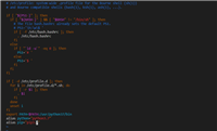
二、代码实现
import numpy as np
import matplotlib.pyplot as plt
from mpl_toolkits.mplot3d import axes3d
from matplotlib import style
#构造数据
def get_data(sample_num=10000):
"""
拟合函数为
y = 5*x1 + 7*x2
:return:
"""
x1 = np.linspace(0, 9, sample_num)
x2 = np.linspace(4, 13, sample_num)
x = np.concatenate(([x1], [x2]), axis=0).t
y = np.dot(x, np.array([5, 7]).t)
return x, y
#梯度下降法
def gd(samples, y, step_size=0.01, max_iter_count=1000):
"""
:param samples: 样本
:param y: 结果value
:param step_size: 每一接迭代的步长
:param max_iter_count: 最大的迭代次数
:param batch_size: 随机选取的相对于总样本的大小
:return:
"""
#确定样本数量以及变量的个数初始化theta值
m, var = samples.shape
theta = np.zeros(2)
y = y.flatten()
#进入循环内
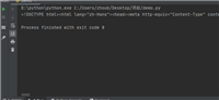
print(samples)
loss = 1
iter_count = 0
iter_list=[]
loss_list=[]
theta1=[]
theta2=[]
#当损失精度大于0.01且迭代此时小于最大迭代次数时,进行
while loss > 0.001 and iter_count < max_iter_count:
loss = 0
#梯度计算
theta1.append(theta[0])
theta2.append(theta[1])
for i in range(m):
h = np.dot(theta,samples[i].t)
#更新theta的值,需要的参量有:步长,梯度
for j in range(len(theta)):
theta[j] = theta[j] - step_size*(1/m)*(h - y[i])*samples[i,j]
#计算总体的损失精度,等于各个样本损失精度之和
for i in range(m):
h = np.dot(theta.t, samples[i])
#每组样本点损失的精度
every_loss = (1/(var*m))*np.power((h - y[i]), 2)
loss = loss + every_loss
print("iter_count: ", iter_count, "the loss:", loss)
iter_list.append(iter_count)
loss_list.append(loss)
iter_count += 1
plt.plot(iter_list,loss_list)
plt.xlabel("iter")
plt.ylabel("loss")
plt.show()
return theta1,theta2,theta,loss_list
def painter3d(theta1,theta2,loss):
style.use('ggplot')
fig = plt.figure()
ax1 = fig.add_subplot(111, projection='3d')
x,y,z = theta1,theta2,loss
ax1.plot_wireframe(x,y,z, rstride=5, cstride=5)
ax1.set_xlabel("theta1")
ax1.set_ylabel("theta2")
ax1.set_zlabel("loss")
plt.show()
def predict(x, theta):
y = np.dot(theta, x.t)
return y
if __name__ == '__main__':
samples, y = get_data()
theta1,theta2,theta,loss_list = gd(samples, y)
print(theta) # 会很接近[5, 7]
painter3d(theta1,theta2,loss_list)
predict_y = predict(theta, [7,8])
print(predict_y)
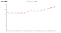
三、绘制的图像如下:
迭代次数与损失精度间的关系图如下:步长为0.01

变量 、
、 与损失函数loss之间的关系:(从初始化之后会一步步收敛到loss满足精度,之后、会变的稳定下来)

下面我们来看一副当步长因子变大后的图像:步长因子为0.5(很明显其收敛速度变缓了)


当步长因子设置为1.8左右时,其损失值已经开始震荡


以上就是本文的全部内容,希望对大家的学习有所帮助,也希望大家多多支持移动技术网。
如对本文有疑问,请在下面进行留言讨论,广大热心网友会与你互动!! 点击进行留言回复

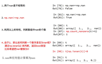
Python 实现将numpy中的nan和inf,nan替换成对应的均值
python爬虫把url链接编码成gbk2312格式过程解析
网友评论