女人心情日记,蔡锷与小凤仙刘晓庆,嫩版leslie
也有些正则方法可以限制回归算法输出结果中系数的影响,其中最常用的两种正则方法是lasso回归和岭回归。
lasso回归和岭回归算法跟常规线性回归算法极其相似,有一点不同的是,在公式中增加正则项来限制斜率(或者净斜率)。这样做的主要原因是限制特征对因变量的影响,通过增加一个依赖斜率a的损失函数实现。
对于lasso回归算法,在损失函数上增加一项:斜率a的某个给定倍数。我们使用tensorflow的逻辑操作,但没有这些操作相关的梯度,而是使用阶跃函数的连续估计,也称作连续阶跃函数,其会在截止点跳跃扩大。一会就可以看到如何使用lasso回归算法。
对于岭回归算法,增加一个l2范数,即斜率系数的l2正则。
# lasso and ridge regression
# lasso回归和岭回归
#
# this function shows how to use tensorflow to solve lasso or
# ridge regression for
# y = ax + b
#
# we will use the iris data, specifically:
# y = sepal length
# x = petal width
# import required libraries
import matplotlib.pyplot as plt
import sys
import numpy as np
import tensorflow as tf
from sklearn import datasets
from tensorflow.python.framework import ops
# specify 'ridge' or 'lasso'
regression_type = 'lasso'
# clear out old graph
ops.reset_default_graph()
# create graph
sess = tf.session()
###
# load iris data
###
# iris.data = [(sepal length, sepal width, petal length, petal width)]
iris = datasets.load_iris()
x_vals = np.array([x[3] for x in iris.data])
y_vals = np.array([y[0] for y in iris.data])
###
# model parameters
###
# declare batch size
batch_size = 50
# initialize placeholders
x_data = tf.placeholder(shape=[none, 1], dtype=tf.float32)
y_target = tf.placeholder(shape=[none, 1], dtype=tf.float32)
# make results reproducible
seed = 13
np.random.seed(seed)
tf.set_random_seed(seed)
# create variables for linear regression
a = tf.variable(tf.random_normal(shape=[1,1]))
b = tf.variable(tf.random_normal(shape=[1,1]))
# declare model operations
model_output = tf.add(tf.matmul(x_data, a), b)
###
# loss functions
###
# select appropriate loss function based on regression type
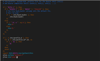
if regression_type == 'lasso':
# declare lasso loss function
# 增加损失函数,其为改良过的连续阶跃函数,lasso回归的截止点设为0.9。
# 这意味着限制斜率系数不超过0.9
# lasso loss = l2_loss + heavyside_step,
# where heavyside_step ~ 0 if a < constant, otherwise ~ 99
lasso_param = tf.constant(0.9)
heavyside_step = tf.truediv(1., tf.add(1., tf.exp(tf.multiply(-50., tf.subtract(a, lasso_param)))))
regularization_param = tf.multiply(heavyside_step, 99.)
loss = tf.add(tf.reduce_mean(tf.square(y_target - model_output)), regularization_param)
elif regression_type == 'ridge':
# declare the ridge loss function
# ridge loss = l2_loss + l2 norm of slope
ridge_param = tf.constant(1.)
ridge_loss = tf.reduce_mean(tf.square(a))
loss = tf.expand_dims(tf.add(tf.reduce_mean(tf.square(y_target - model_output)), tf.multiply(ridge_param, ridge_loss)), 0)
else:
print('invalid regression_type parameter value',file=sys.stderr)
###
# optimizer
###
# declare optimizer
my_opt = tf.train.gradientdescentoptimizer(0.001)
train_step = my_opt.minimize(loss)
###
# run regression
###
# initialize variables
init = tf.global_variables_initializer()
sess.run(init)
# training loop
loss_vec = []
for i in range(1500):
rand_index = np.random.choice(len(x_vals), size=batch_size)
rand_x = np.transpose([x_vals[rand_index]])
rand_y = np.transpose([y_vals[rand_index]])
sess.run(train_step, feed_dict={x_data: rand_x, y_target: rand_y})
temp_loss = sess.run(loss, feed_dict={x_data: rand_x, y_target: rand_y})
loss_vec.append(temp_loss[0])
if (i+1)%300==0:
print('step #' + str(i+1) + ' a = ' + str(sess.run(a)) + ' b = ' + str(sess.run(b)))
print('loss = ' + str(temp_loss))
print('\n')
###
# extract regression results
###
# get the optimal coefficients
[slope] = sess.run(a)
[y_intercept] = sess.run(b)
# get best fit line
best_fit = []
for i in x_vals:
best_fit.append(slope*i+y_intercept)
###
# plot results
###
# plot regression line against data points
plt.plot(x_vals, y_vals, 'o', label='data points')
plt.plot(x_vals, best_fit, 'r-', label='best fit line', linewidth=3)
plt.legend(loc='upper left')
plt.title('sepal length vs pedal width')
plt.xlabel('pedal width')
plt.ylabel('sepal length')
plt.show()
# plot loss over time
plt.plot(loss_vec, 'k-')
plt.title(regression_type + ' loss per generation')
plt.xlabel('generation')
plt.ylabel('loss')
plt.show()
输出结果:
step #300 a = [[ 0.77170753]] b = [[ 1.82499862]]
loss = [[ 10.26473045]]
step #600 a = [[ 0.75908542]] b = [[ 3.2220633]]
loss = [[ 3.06292033]]
step #900 a = [[ 0.74843585]] b = [[ 3.9975822]]
loss = [[ 1.23220456]]
step #1200 a = [[ 0.73752165]] b = [[ 4.42974091]]
loss = [[ 0.57872057]]
step #1500 a = [[ 0.72942668]] b = [[ 4.67253113]]
loss = [[ 0.40874988]]


通过在标准线性回归估计的基础上,增加一个连续的阶跃函数,实现lasso回归算法。由于阶跃函数的坡度,我们需要注意步长,因为太大的步长会导致最终不收敛。
以上就是本文的全部内容,希望对大家的学习有所帮助,也希望大家多多支持移动技术网。
如对本文有疑问,请在下面进行留言讨论,广大热心网友会与你互动!! 点击进行留言回复


Python 实现将numpy中的nan和inf,nan替换成对应的均值

python爬虫把url链接编码成gbk2312格式过程解析
网友评论